Topic Modeling
Autonomy
Digital Media
Self-Determination
This is a documentation of the code that was used to calculate the topic model. (Some of) the code will not be evaluated in this document but refer to a saved version of the topic model and the lemmatised tokens to save computing time and to ensure reproducibility.
Load Data
Load the cleaned abstracts.
Lemmatise
Further Cleaning
# combine lemmas with article information
lemmas <- lemmas %>% mutate(doc_id = as.numeric(doc_id))
lemmas <- left_join(x = lemmas, y = clean_papers)

# keep only nouns
lemmas <- lemmas %>% filter(upos == "NOUN")

# summarise on document level
docs <- lemmas %>%
  group_by(doc_id) %>%
  summarise(lemmatised_abstract = paste(lemma, collapse = " "),
            across(names(clean_papers)[-1])) %>%
  distinct() %>%
  relocate(lemmatised_abstract, .after = abstract) %>%
  ungroup()
# check again if abstract of covariates of interest have missing values
table(is.na(docs$lemmatised_abstract))
FALSE
 1744
FALSE
 1744
FALSE
 1744
# clean again
docs <- docs %>%
# clean punctuation
mutate(clean_abstract = str_replace_all(lemmatised_abstract, "[:punct:]", "")) %>%
# clean symbols
mutate(clean_abstract = str_replace_all(clean_abstract, "[:symbol:]", "")) %>%
# clean numbers
mutate(clean_abstract = str_replace_all(clean_abstract, "[:digit:]", "")) %>%
#clean hashtags
mutate(clean_abstract = str_replace_all(clean_abstract, "#\\w+", "")) %>%
# clean unnecessary white spaces
mutate(clean_abstract = str_squish(clean_abstract)) %>%
# move clean abstract to front and remove lemmatised abstract variable
relocate(clean_abstract, .after = abstract) %>%
select(-lemmatised_abstract)# check again if abstract of covariates of interest have missing values
table(is.na(docs$clean_abstract))
FALSE
 1744
FALSE
 1744
FALSE
 1744
# load words that are frequently used in abstracts of research articles
common_words <- read_rds("data/common_words.rds")
common_words [1] "data" "condition"
[3] "survey" "factor"
[5] "sample" "result"
[7] "experiment" "variable"
[9] "questionnaire" "regression"
[11] "respondent" "scale"
[13] "study" "paper"
[15] "approach" "concept"
[17] "framework" "analysis"
[19] "theoretical" "develop"
[21] "discuss" "base"
[23] "assessment" "perspective"
[25] "question" "main"
[27] "methodology" "aim"
[29] "theory" "apply"
[31] "purpose" "reference"
[33] "context" "establish"
[35] "idea" "field"
[37] "level" "understanding"
[39] "focus" "design"
[41] "highlight" "potential"
[43] "basis" "evaluation"
[45] "methods" "identify"
[47] "define" "follow"
[49] "discussion" "extensive"
[51] "practical" "aspect"
[53] "propose" "conclusion"
[55] "classical" "article"
[57] "facilitate" "researchers"
[59] "possibility" "literature"
[61] "content" "implication"
[63] "construction" "emphasize"
[65] "empirical" "form"
[67] "conceptual" "paradigm"
[69] "address" "key"
[71] "interdisciplinary" "review"
[73] "adopt" "analyse"
[75] "goal" "expect"
[77] "implementation" "change"
[79] "description" "alternative"
[81] "scope" "investigation"
[83] "step" "contemporary"
[85] "demonstrate" "proposal"
[87] "reflect" "characteristic"
[89] "draw" "sense"
[91] "account" "introduce"
[93] "outline" "degree"
[95] "definition" "emphasis"
[97] "start" "understand"
[99] "interpretation" "list"
[101] "support" "attempt"
[103] "author" "investigate"
[105] "center" "formal"
[107] "topic" "bring"
[109] "examine" "model"
[111] "enable" "view"
[113] "debate" "crucial"
[115] "reflection" "involve"
[117] "overcome" "approaches"
[119] "collaborative" "conception"
[121] "manage" "contribution"
[123] "suitable" "stage"
[125] "abstract" "introduction"
[127] "collaboration" "refer"
[129] "object" "raise"
[131] "core" "incorporate"
[133] "include" "organize"
[135] "map" "broad"
[137] "method" "exist"
[139] "critique" "seek"
[141] "logic" "sciences"
[143] "source" "evidence"
[145] "feedback" "notion"
[147] "produce" "component"
[149] "relevant" "provide"
[151] "role" "external"
[153] "fit" "concern"
[155] "remain" "qualitative"
[157] "objective" "foundation"
[159] "designmethodologyapproach" "comparison"
[161] "critically" "explanation"
[163] "scenario" "finding"
[165] "explain" "interaction"
[167] "exploratory" "experimental"
[169] "construct" "theories"
[171] "exploration" "measure"
[173] "findings" # unnest tokens and remove stopwords, typical words for research articles
# and all words related to autonomy
tidy_docs <- docs %>%
unnest_tokens(word, clean_abstract, token = "words", to_lower = TRUE) %>%
anti_join(get_stopwords(language = "en", source="stopwords-iso")) %>%
filter(!str_detect(word, "autonom")) %>% # remove "autonomy" because this word should be in all topics
filter(!word %in% common_words) %>% # remove common research article words
add_count(word) %>%
filter(n > 20) %>% # remove very infrequent terms
select(-n)
# sparse matrix
sparse_docs <- tidy_docs %>%
count(doc_id, word) %>%
cast_sparse(doc_id, word, n)Topic Model
# define parameters
min <- 5
max <- 100
steps <- 1
k_range <- seq(min, max, steps)

# plan multiprocessing
plan(multisession, workers = 8)

# set seed
set.seed(42)

# calculate many models
many_models <- tibble(K = k_range) %>%
  mutate(topic_model = future_map(K,
                                  ~ stm(sparse_docs,
                                        prevalence =~ year + main_concept,
                                        data = docs,
                                        gamma.prior = "L1",
                                        K = .,
                                        verbose = FALSE),
         .options = furrr_options(seed = 42),
         .progress = TRUE))
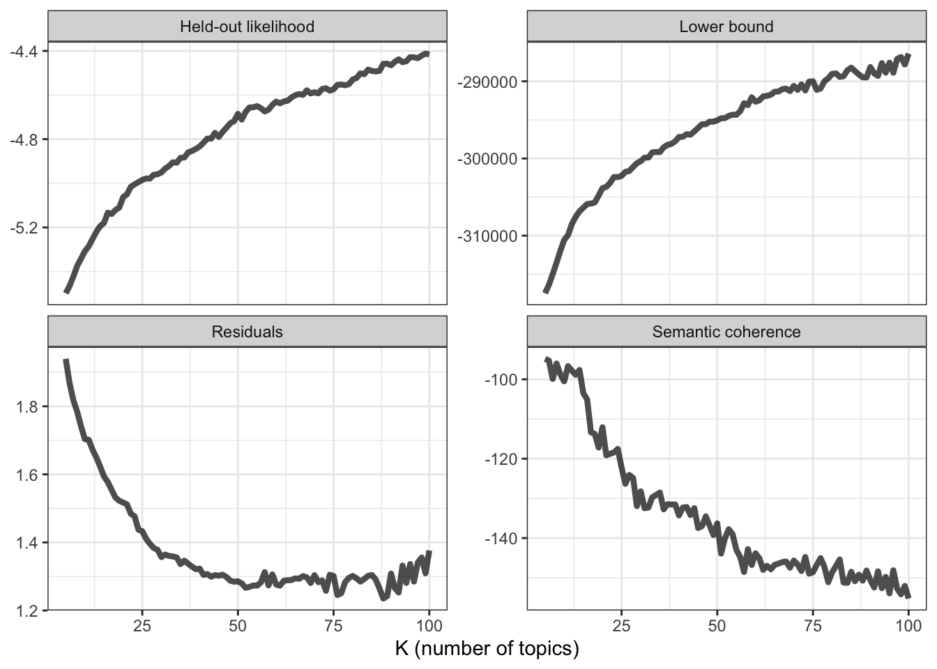
Model Diagnostics
# make heldout
heldout <- make.heldout(sparse_docs, seed = 42)

# calculate diagnostics
k_result <- many_models %>%
  mutate(exclusivity = map(topic_model, exclusivity),
         semantic_coherence = map(topic_model, semanticCoherence, sparse_docs),
         eval_heldout = map(topic_model, eval.heldout, heldout$missing),
         residual = map(topic_model, checkResiduals, sparse_docs),
         bound =  map_dbl(topic_model, function(x) max(x$convergence$bound)),
         lfact = map_dbl(topic_model, function(x) lfactorial(x$settings$dim$K)),
         lbound = bound + lfact,
         iterations = map_dbl(topic_model, function(x) length(x$convergence$bound)))

# plot diagnostics
k_result %>%
  transmute(K,
            `Lower bound` = lbound,
            Residuals = map_dbl(residual, "dispersion"),
            `Semantic coherence` = map_dbl(semantic_coherence, mean),
            `Held-out likelihood` = map_dbl(eval_heldout, "expected.heldout")) %>%
  gather(Metric, Value, -K) %>%
  ggplot(aes(K, Value)) +
  geom_line(size = 1.5, alpha = 0.7, show.legend = FALSE) +
  facet_wrap(~Metric, scales = "free_y") +
  labs(x = "K (number of topics)",
       y = NULL) +
  theme_bw()
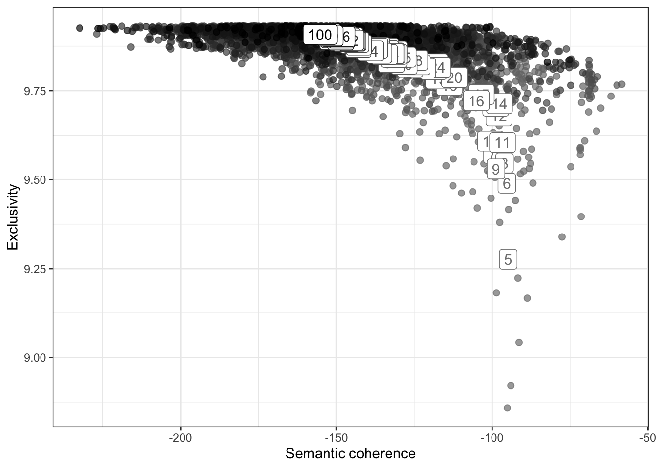
# define range to check for exclusivity and semantic coherence
range <- seq(5, 100, 1)

# calculate exclusivity and semantic coherence
group_means <- k_result %>%
  select(K, exclusivity, semantic_coherence) %>%
  filter(K %in% range) %>%
  unnest(cols = c(exclusivity, semantic_coherence)) %>%
  mutate(K = as.factor(K)) %>%
  group_by(K) %>%
  summarise(
    exclusivity = mean(exclusivity),
    semantic_coherence = mean(semantic_coherence)
  )

# plot semantic coherence and exclusivity
k_result %>%
  select(K, exclusivity, semantic_coherence) %>%
  filter(K %in% range) %>%
  unnest(cols = c(exclusivity, semantic_coherence)) %>%
  mutate(K = as.factor(K)) %>%
  ggplot(aes(semantic_coherence, exclusivity, z = K, color = K)) +
  geom_point(size = 2, alpha = 0.7) +
  geom_label(data = group_means, label = group_means$K, size = 4, show.legend = FALSE) +
  labs(x = "Semantic coherence",
       y = "Exclusivity") +
  theme_bw() +
  theme(legend.position = "none") +
  scale_color_grey(start = .5, end = 0)
# extract k = 14 model
topic_model <- k_result %>%
  filter(K == 14) %>%
  pull(topic_model) %>%
  .[[1]]

topic_model
A topic model with 14 topics, 1744 documents and a 652 word dictionary.Inspect Model
# beta (probabilities that each word is generated from each topic)
td_beta <- tidy(topic_model)
td_beta
# A tibble: 9,128 × 3
topic term beta
<int> <chr> <dbl>
1 1 absence 5.38e- 4
2 2 absence 1.76e- 3
3 3 absence 7.69e-12
4 4 absence 1.28e-13
5 5 absence 5.54e- 9
6 6 absence 1.08e- 4
7 7 absence 4.17e-23
8 8 absence 1.05e- 5
9 9 absence 1.94e- 3
10 10 absence 5.66e- 7
# … with 9,118 more rows
# ℹ Use `print(n = ...)` to see more rows# gamma (probabilities that each document is generated from each topic)
td_gamma <- tidy(topic_model, matrix = "gamma",
document_names = rownames(sparse_docs))
td_gamma# A tibble: 24,416 × 3
document topic gamma
<chr> <int> <dbl>
1 1 1 0.00925
2 2 1 0.00573
3 3 1 0.0268
4 4 1 0.00456
5 5 1 0.0174
6 6 1 0.0332
7 7 1 0.0235
8 8 1 0.0212
9 9 1 0.00209
10 10 1 0.00303
# … with 24,406 more rows
# ℹ Use `print(n = ...)` to see more rows# top terms
top_terms <- td_beta %>%
arrange(beta) %>%
group_by(topic) %>%
top_n(20, beta) %>%
arrange(-beta) %>%
select(topic, term) %>%
summarise(terms = list(term)) %>%
mutate(terms = map(terms, paste, collapse = ", ")) %>%
unnest(cols = c(terms))
top_terms# A tibble: 14 × 2
topic terms
<int> <chr>
1 1 life, woman, child, family, parent, time, sex, phone, image, gender, a…
2 2 internet, law, freedom, privacy, principle, rights, issue, protection,…
3 3 government, management, policy, governance, development, service, busi…
4 4 student, school, teacher, college, class, classroom, perception, scien…
5 5 employee, job, worker, innovation, relationship, performance, organiza…
6 6 learner, language, teaching, teacher, technology, internet, learning, …
7 7 internet, relationship, adolescent, behavior, consumer, dimension, add…
8 8 participant, motivation, competence, satisfaction, relatedness, activi…
9 9 health, care, patient, people, nurse, healthcare, professional, decisi…
10 10 media, network, community, space, identity, culture, platform, practic…
11 11 team, agent, time, task, target, communication, failure, situation, pr…
12 12 technology, user, communication, people, device, service, tool, applic…
13 13 education, process, institution, skill, development, university, train…
14 14 control, intelligence, knowledge, solution, environment, issue, trust,…# top gamma terms
gamma_terms <- td_gamma %>%
group_by(topic) %>%
summarise(gamma = mean(gamma)) %>%
arrange(desc(gamma)) %>%
left_join(top_terms, by = "topic") %>%
mutate(topic = paste0("Topic ", topic),
topic = reorder(topic, gamma))
gamma_terms# A tibble: 14 × 3
topic gamma terms
<fct> <dbl> <chr>
1 Topic 6 0.111 learner, language, teaching, teacher, technology, internet, …
2 Topic 2 0.102 internet, law, freedom, privacy, principle, rights, issue, p…
3 Topic 10 0.0996 media, network, community, space, identity, culture, platfor…
4 Topic 12 0.0864 technology, user, communication, people, device, service, to…
5 Topic 4 0.0706 student, school, teacher, college, class, classroom, percept…
6 Topic 14 0.0701 control, intelligence, knowledge, solution, environment, iss…
7 Topic 3 0.0677 government, management, policy, governance, development, ser…
8 Topic 13 0.0669 education, process, institution, skill, development, univers…
9 Topic 7 0.0632 internet, relationship, adolescent, behavior, consumer, dime…
10 Topic 5 0.0607 employee, job, worker, innovation, relationship, performance…
11 Topic 8 0.0598 participant, motivation, competence, satisfaction, relatedne…
12 Topic 1 0.0542 life, woman, child, family, parent, time, sex, phone, image,…
13 Topic 9 0.0539 health, care, patient, people, nurse, healthcare, profession…
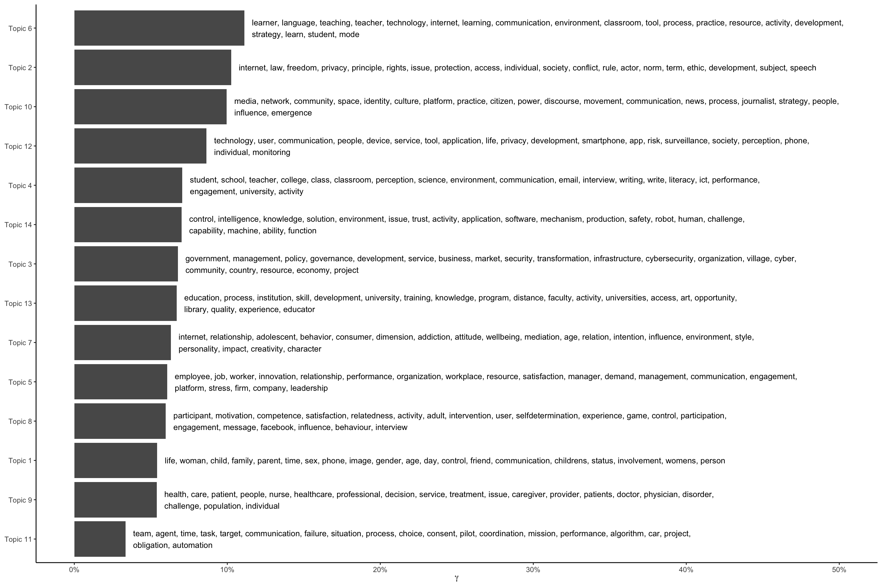
14 Topic 11 0.0334 team, agent, time, task, target, communication, failure, sit…# plot top gamma terms
gamma_terms %>%
ggplot(aes(topic, gamma, label = str_wrap(terms, width = 170))) +
geom_col(show.legend = FALSE) +
geom_text(hjust = 0, nudge_y = 0.005, size = 3.5) +
coord_flip() +
scale_y_continuous(labels = scales::percent_format(), limits = c(0, .5)) +
labs(x = NULL, y = expression(gamma)) +
theme_classic()
# get top topic (highest probability) per doc
top_classification <- td_gamma %>%
  group_by(document) %>%
  top_n(1, gamma) %>%
  ungroup() %>%
  mutate(doc_id = as.numeric(document))

top_classification
# A tibble: 1,744 × 4
document topic gamma doc_id
<chr> <int> <dbl> <dbl>
1 13 1 0.401 13
2 16 1 0.429 16
3 37 1 0.675 37
4 38 1 0.604 38
5 42 1 0.358 42
6 51 1 0.531 51
7 98 1 0.608 98
8 120 1 0.366 120
9 150 1 0.682 150
10 156 1 0.270 156
# … with 1,734 more rows
# ℹ Use `print(n = ...)` to see more rows# add top topic (highest probability) to docs
topic_docs <- inner_join(docs, top_classification) %>%
relocate(topic, gamma, .after = doc_id)
# save abstracts by topic
# digital policy
digital_policy <- topic_docs %>%
filter(topic == 2 | topic == 12 | topic == 3)
digital_pedagogy <- topic_docs %>%
filter(topic == 6 | topic == 4 | topic == 13)
digital_media_use <- topic_docs %>%
filter(topic == 7 | topic == 8)
machine_autonomy <- topic_docs %>%
filter(topic == 14 | topic == 11)
digital_power_structures <- topic_docs %>%
filter(topic == 10)
digital_workplace <- topic_docs %>%
filter(topic == 5)
adolescence <- topic_docs %>%
filter(topic == 1)
digital_healthcare <- topic_docs %>%
filter(topic == 9)
# check if paper cites sdt
sdt_papers <- read_rds("data/sdt_papers.rds")
is_sdt_paper <-
topic_docs %>%
mutate(
topic = str_c("Topic ", topic) %>% as_factor(),
is_sdt_paper = if_else(doc_id %in% sdt_papers$doc_id, 1, 0)
) %>%
group_by(topic) %>%
summarise(percent_sdt = mean(is_sdt_paper))
# get top concepts by topic
top_topic_concepts <- topic_docs %>%
select(-concept_id, -concept_score, -concept_lecel, -concept_url) %>%
unnest(all_concepts) %>%
filter(concept_name != "Autonomy") %>%
group_by(doc_id, topic) %>%
arrange(concept_lecel, .by_group = TRUE) %>%
group_by(topic, concept_name) %>%
summarise(n = n()) %>%
arrange(desc(n), .by_group = TRUE) %>%
filter(row_number() %in% 1:3) %>%
mutate(
top_topic_concepts = str_flatten(concept_name, collapse = ", "),
topic = str_c("Topic ", topic) %>% as_factor()) %>%
nest(all_concepts = c(concept_name, n))
top_topic_concepts <- left_join(gamma_terms, top_topic_concepts)
# add manual topic labels after inspecting concepts and top words
topic_labels <-
tribble(
~ topic, ~ label,
"Topic 1", "Adolescence",
"Topic 2", "Digital Policy",
"Topic 3", "Digital Policy",
"Topic 4", "Digital Pedagogy",
"Topic 5", "Digital Workplace",
"Topic 6", "Digital Pedagogy",
"Topic 7", "Digital Media Use",
"Topic 8", "Digital Media Use",
"Topic 9", "Digital Healthcare",
"Topic 10", "Digital Power Structures",
"Topic 11", "Machine Autonomy",
"Topic 12", "Digital Policy",
"Topic 13", "Digital Pedagogy",
"Topic 14", "Machine Autonomy",
) %>%
mutate(
topic = as.factor(topic),
label = as.factor(label)
)
# order by sum of gamma by manual topic
top_topic_concepts_plot <- left_join(top_topic_concepts, topic_labels) %>%
left_join(is_sdt_paper) %>%
group_by(label) %>%
mutate(
order = sum(gamma)
) %>%
ungroup() %>%
mutate(label = fct_reorder(label, order, .desc = TRUE))
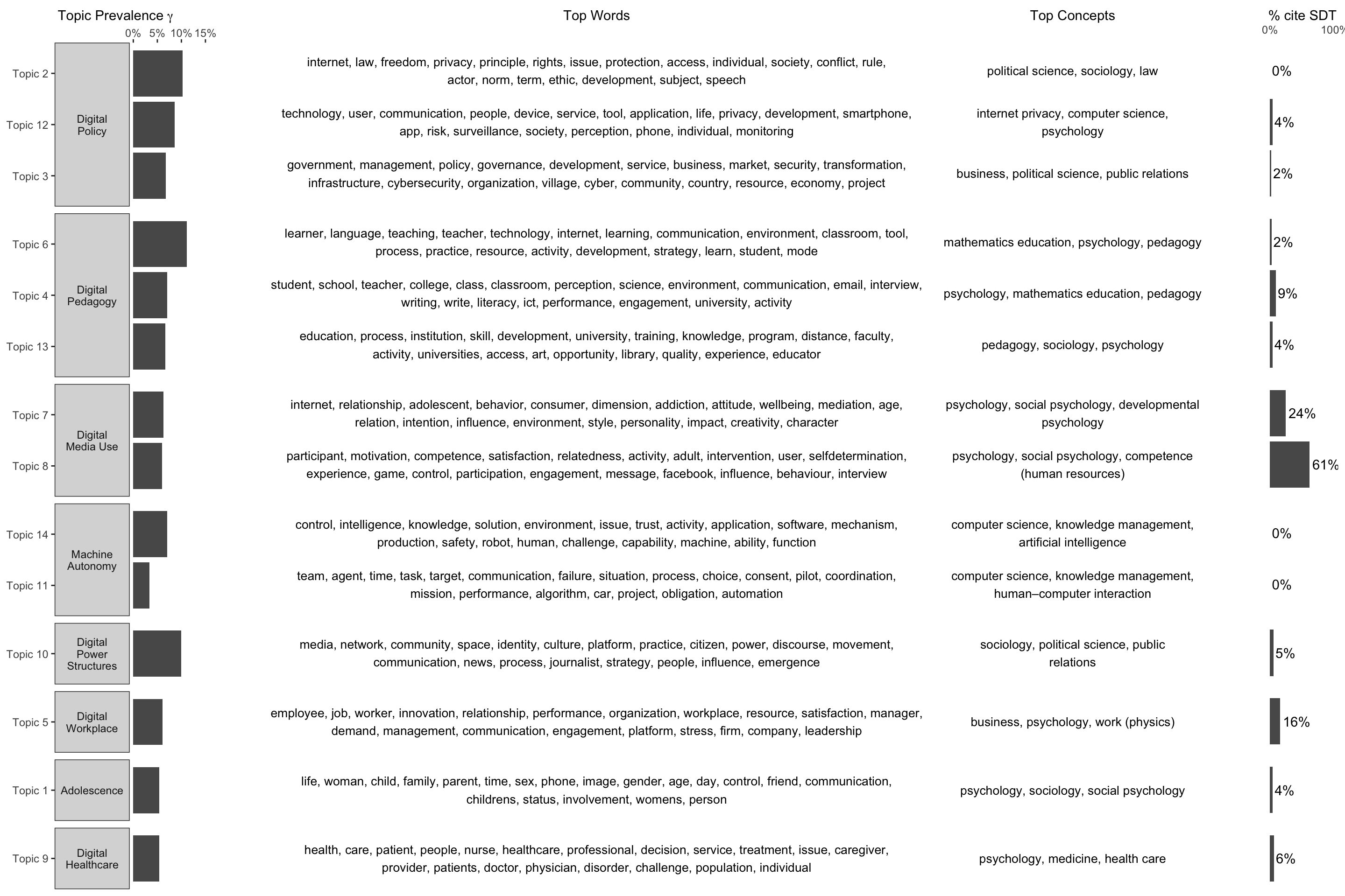
# plot
p1 <- top_topic_concepts_plot %>%
ggplot(aes(topic, gamma)) +
geom_col(show.legend = FALSE) +
coord_flip() +
scale_y_continuous(labels = scales::percent_format(),
limits = c(0, .15), position = "right",
breaks = c(0, .05, .1, .15)) +
labs(x = NULL, y = expression("Topic Prevalence " * gamma)) +
facet_grid(rows = vars(label), scales = "free_y", space = "free_y",
labeller = labeller(label = label_wrap_gen(10)),
switch = "y") +
theme_bw() +
theme(strip.text.y.left = element_text(angle = 0),
axis.title.x = element_text(hjust = 2),
panel.grid = element_blank(),
panel.border = element_blank())
p2 <- top_topic_concepts_plot %>%
ggplot(aes(topic, gamma)) +
geom_text(aes(label = str_wrap(terms, width = 120), y = 0), hjust = 0.5, size = 3.5) +
coord_flip() +
scale_y_continuous(position = "right") +
facet_grid(rows = vars(label), scales = "free_y", space = "free_y") +
theme_bw() +
ylab("Top Words") +
theme(axis.line = element_blank(),
axis.text.x = element_text(colour = "#ffffff"),
axis.text.y = element_text(colour = "#ffffff"),
axis.ticks = element_blank(),
axis.title.y = element_blank(),
strip.background.y = element_blank(),
strip.text.y = element_blank(),
panel.grid = element_blank(),
panel.border = element_blank())
p3 <- top_topic_concepts_plot %>%
ggplot(aes(topic, gamma)) +
geom_text(aes(label = str_wrap(str_to_lower(top_topic_concepts), width = 45), y = 0),
hjust = 0.5, size = 3.5) +
coord_flip() +
scale_y_continuous(position = "right") +
facet_grid(rows = vars(label), scales = "free_y", space = "free_y") +
theme_bw() +
ylab("Top Concepts") +
theme(axis.line = element_blank(),
axis.text.x = element_text(colour = "#ffffff"),
axis.text.y = element_blank(),
axis.ticks = element_blank(),
axis.title.y = element_blank(),
strip.background.y = element_blank(),
strip.text.y = element_blank(),
panel.grid = element_blank(),
panel.border = element_blank())
p4 <- top_topic_concepts_plot %>%
ggplot(aes(topic, percent_sdt)) +
geom_col(show.legend = FALSE) +
geom_text(aes(label = str_c(round(percent_sdt * 100, 0), "%")), hjust = -.1) +
coord_flip() +
scale_y_continuous(labels = scales::percent_format(),
limits = c(0, 1), position = "right",
breaks = c(0, 1)) +
labs(x = NULL, y = "% cite SDT") +
facet_grid(rows = vars(label), scales = "free_y", space = "free_y",
labeller = labeller(label = label_wrap_gen(10)),
switch = "y") +
theme_bw() +
theme(axis.line = element_blank(),
# axis.text.x = element_text(colour = "#ffffff"),
axis.text.y = element_text(colour = "#ffffff"),
axis.ticks = element_blank(),
axis.title.y = element_blank(),
strip.background.y = element_blank(),
strip.text.y = element_blank(),
panel.grid = element_blank(),
panel.border = element_blank())
ggarrange(p1, p2, p3, p4,
ncol = 4, nrow = 1,
widths = c(.65 , 2.15, .85, .4))