SDT Focus
Autonomy
Digital Media
Self-Determination
This is a documentation of the code that was used to calculate the topic model. (Some of) the code will not be evaluated in this document but refer to a saved version of the topic model and the lemmatised tokens to save computing time and to ensure reproducibility.
Load Data
Load the cleaned abstracts.
Filter SDT-Papers
# extract referenced papers
cited_paper_ids <-
  clean_papers %>%
  unnest(referenced_works) %>%
  mutate(
    ref_oaid = str_extract(referenced_works, "(?<=https\\://openalex\\.org/)(.*)"),
    .after = referenced_works
    ) %>%
  distinct(ref_oaid) %>%
  pull(ref_oaid)

# get cited papers from API
if (!file.exists("data/cited_papers.rds")) {
  cited_paper_ids %>%
    sample(1) %>%
    oa_fetch(identifier = ., entity = "works") %>%
    mutate(
      oaid = str_extract(id, "(?<=https\\://openalex\\.org/)(.*)")
    ) %>%
    write_rds("data/cited_papers.rds")
}

replicate(1000, {
  todo <-
    cited_paper_ids %>%
    as_tibble() %>%
    rename(oaid = value) %>%
    anti_join(., read_rds("data/cited_papers.rds")) %>%
    slice_sample(n = 50) %>%
    pull(oaid)

    if(length(todo)==0) return(TRUE)

    todo %>%
    oa_fetch(identifier = ., entity = "works") %>%
    mutate(
      oaid = str_extract(id, "(?<=https\\://openalex\\.org/)(.*)")
    ) %>%
    bind_rows(read_rds("data/cited_papers.rds")) %>%
    distinct() %>%
    write_rds("data/cited_papers.rds")
})

read_rds("data/cited_papers.rds") %>%
  distinct() %>%
  write_rds("data/cited_papers.rds")
# extract related papers
related_paper_ids <-
clean_papers %>%
unnest(related_works) %>%
mutate(
rel_oaid = str_extract(related_works, "(?<=https\\://openalex\\.org/)(.*)"),
.after = related_works
) %>%
distinct(rel_oaid) %>%
pull(rel_oaid)
# get related papers from API
if (!file.exists("data/related_papers.rds")) {
related_paper_ids %>%
sample(1) %>%
oa_fetch(identifier = ., entity = "works") %>%
mutate(
oaid = str_extract(id, "(?<=https\\://openalex\\.org/)(.*)")
) %>%
write_rds("data/related_papers.rds")
}
replicate(1000, {
todo <-
related_paper_ids %>%
as_tibble() %>%
rename(oaid = value) %>%
anti_join(., read_rds("data/related_papers.rds")) %>%
slice_sample(n = 50) %>%
pull(oaid)
if(length(todo)==0) return(TRUE)
todo %>%
oa_fetch(identifier = ., entity = "works") %>%
mutate(
oaid = str_extract(id, "(?<=https\\://openalex\\.org/)(.*)")
) %>%
bind_rows(read_rds("data/related_papers.rds")) %>%
distinct() %>%
write_rds("data/related_papers.rds")
})
read_rds("data/related_papers.rds") %>%
distinct() %>%
write_rds("data/related_papers.rds")# extract papers authored by Deci and/or Ryan
deci_ryan <-
bind_rows(cited_papers, related_papers) %>%
unnest(author) %>%
mutate(
au_id = str_extract(au_id, "(?<=https\\://openalex\\.org/)(.*)")
) %>%
filter(
au_id %in% c("A1906028136", # Edward L. Deci
"A2166335463" # Richard M. Ryan
)
) %>%
distinct(oaid) %>%
pull(oaid)
# extract SDT related papers
ref_sdt_papers <-
clean_papers %>%
unnest(referenced_works) %>%
mutate(
ref_oaid = str_extract(referenced_works, "(?<=https\\://openalex\\.org/)(.*)"),
.after = referenced_works
) %>%
filter(ref_oaid %in% deci_ryan) %>%
nest(referenced_works = c(referenced_works, ref_oaid))
rel_sdt_papers <-
clean_papers %>%
unnest(related_works) %>%
mutate(
rel_oaid = str_extract(related_works, "(?<=https\\://openalex\\.org/)(.*)"),
.after = related_works
) %>%
filter(rel_oaid %in% deci_ryan) %>%
nest(related_works = c(related_works, rel_oaid))
sdt_papers <-
bind_rows(ref_sdt_papers, rel_sdt_papers) %>%
distinct(doc_id, .keep_all = TRUE) %>%
arrange(doc_id)
# save
sdt_papers %>%
write_rds("data/sdt_papers.rds")Lemmatise
Further Cleaning
# combine lemmas with article information
lemmas <- lemmas %>% mutate(doc_id = as.numeric(doc_id))
lemmas <- left_join(x = lemmas,
                    y = sdt_papers %>% rename(old_doc_id = doc_id) %>% rowid_to_column(var = "doc_id"))

# keep only nouns
lemmas <- lemmas %>% filter(upos == "NOUN")

# summarise on document level
docs <- lemmas %>%
  group_by(doc_id) %>%
  summarise(lemmatised_abstract = paste(lemma, collapse = " "),
            across(names(sdt_papers)[-1])) %>%
  distinct() %>%
  relocate(lemmatised_abstract, .after = abstract) %>%
  ungroup()
# check again if abstract of covariates of interest have missing values
table(is.na(docs$lemmatised_abstract))
FALSE
  149
FALSE
  149
FALSE
  149
# clean again
docs <- docs %>%
# clean punctuation
mutate(clean_abstract = str_replace_all(lemmatised_abstract, "[:punct:]", "")) %>%
# clean symbols
mutate(clean_abstract = str_replace_all(clean_abstract, "[:symbol:]", "")) %>%
# clean numbers
mutate(clean_abstract = str_replace_all(clean_abstract, "[:digit:]", "")) %>%
#clean hashtags
mutate(clean_abstract = str_replace_all(clean_abstract, "#\\w+", "")) %>%
# clean unnecessary white spaces
mutate(clean_abstract = str_squish(clean_abstract)) %>%
# move clean abstract to front and remove lemmatised abstract variable
relocate(clean_abstract, .after = abstract) %>%
select(-lemmatised_abstract)# check again if abstract of covariates of interest have missing values
table(is.na(docs$clean_abstract))
FALSE
  149
FALSE
  149
FALSE
  149
# load words that are frequently used in abstracts of research articles
common_words <- read_rds("data/common_words.rds")
common_words [1] "data" "condition"
[3] "survey" "factor"
[5] "sample" "result"
[7] "experiment" "variable"
[9] "questionnaire" "regression"
[11] "respondent" "scale"
[13] "study" "paper"
[15] "approach" "concept"
[17] "framework" "analysis"
[19] "theoretical" "develop"
[21] "discuss" "base"
[23] "assessment" "perspective"
[25] "question" "main"
[27] "methodology" "aim"
[29] "theory" "apply"
[31] "purpose" "reference"
[33] "context" "establish"
[35] "idea" "field"
[37] "level" "understanding"
[39] "focus" "design"
[41] "highlight" "potential"
[43] "basis" "evaluation"
[45] "methods" "identify"
[47] "define" "follow"
[49] "discussion" "extensive"
[51] "practical" "aspect"
[53] "propose" "conclusion"
[55] "classical" "article"
[57] "facilitate" "researchers"
[59] "possibility" "literature"
[61] "content" "implication"
[63] "construction" "emphasize"
[65] "empirical" "form"
[67] "conceptual" "paradigm"
[69] "address" "key"
[71] "interdisciplinary" "review"
[73] "adopt" "analyse"
[75] "goal" "expect"
[77] "implementation" "change"
[79] "description" "alternative"
[81] "scope" "investigation"
[83] "step" "contemporary"
[85] "demonstrate" "proposal"
[87] "reflect" "characteristic"
[89] "draw" "sense"
[91] "account" "introduce"
[93] "outline" "degree"
[95] "definition" "emphasis"
[97] "start" "understand"
[99] "interpretation" "list"
[101] "support" "attempt"
[103] "author" "investigate"
[105] "center" "formal"
[107] "topic" "bring"
[109] "examine" "model"
[111] "enable" "view"
[113] "debate" "crucial"
[115] "reflection" "involve"
[117] "overcome" "approaches"
[119] "collaborative" "conception"
[121] "manage" "contribution"
[123] "suitable" "stage"
[125] "abstract" "introduction"
[127] "collaboration" "refer"
[129] "object" "raise"
[131] "core" "incorporate"
[133] "include" "organize"
[135] "map" "broad"
[137] "method" "exist"
[139] "critique" "seek"
[141] "logic" "sciences"
[143] "source" "evidence"
[145] "feedback" "notion"
[147] "produce" "component"
[149] "relevant" "provide"
[151] "role" "external"
[153] "fit" "concern"
[155] "remain" "qualitative"
[157] "objective" "foundation"
[159] "designmethodologyapproach" "comparison"
[161] "critically" "explanation"
[163] "scenario" "finding"
[165] "explain" "interaction"
[167] "exploratory" "experimental"
[169] "construct" "theories"
[171] "exploration" "measure"
[173] "findings" # unnest tokens and remove stopwords, typical words for research articles
# and all words related to autonomy
tidy_docs <- docs %>%
unnest_tokens(word, clean_abstract, token = "words", to_lower = TRUE) %>%
anti_join(get_stopwords(language = "en", source="stopwords-iso")) %>%
filter(!str_detect(word, "autonom")) %>% # remove "autonomy" because this word should be in all topics
filter(!word %in% common_words) %>% # remove common research article words
add_count(word) %>%
filter(n >= 5) %>% # remove very infrequent terms
select(-n)
# sparse matrix
sparse_docs <- tidy_docs %>%
count(doc_id, word) %>%
cast_sparse(doc_id, word, n)Topic Model
# define parameters
min <- 5
max <- 100
steps <- 1
k_range <- seq(min, max, steps)

# plan multiprocessing
plan(multisession, workers = 8)

# set seed
set.seed(42)

# calculate many models
many_models <- tibble(K = k_range) %>%
  mutate(topic_model = future_map(K,
                                  ~ stm(sparse_docs,
                                        prevalence =~ year + main_concept,
                                        data = docs,
                                        gamma.prior = "L1",
                                        K = .,
                                        verbose = FALSE),
         .options = furrr_options(seed = 42),
         .progress = TRUE))
Model Diagnostics
# make heldout
heldout <- make.heldout(sparse_docs, seed = 42)

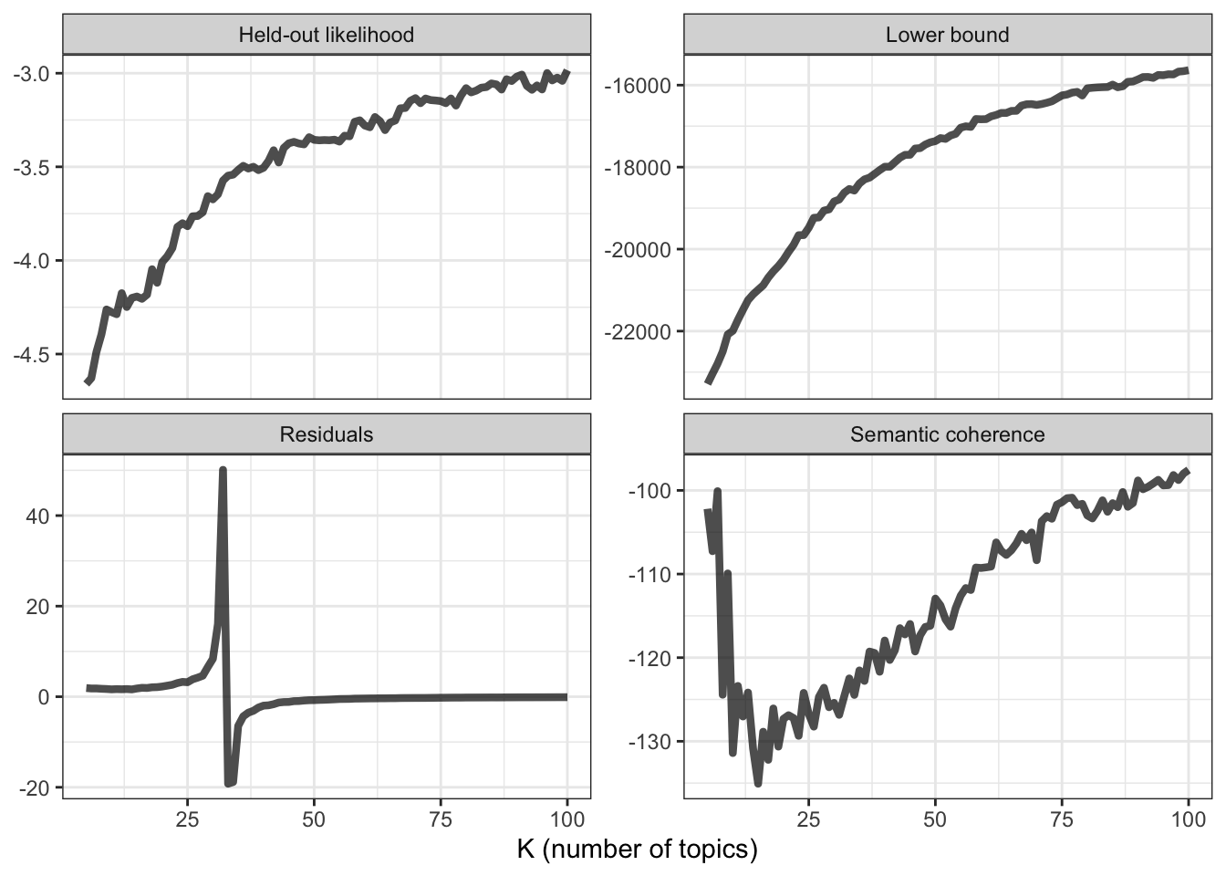
# calculate diagnostics
k_result <- many_models %>%
  mutate(exclusivity = map(topic_model, exclusivity),
         semantic_coherence = map(topic_model, semanticCoherence, sparse_docs),
         eval_heldout = map(topic_model, eval.heldout, heldout$missing),
         residual = map(topic_model, checkResiduals, sparse_docs),
         bound =  map_dbl(topic_model, function(x) max(x$convergence$bound)),
         lfact = map_dbl(topic_model, function(x) lfactorial(x$settings$dim$K)),
         lbound = bound + lfact,
         iterations = map_dbl(topic_model, function(x) length(x$convergence$bound)))

# plot diagnostics
k_result %>%
  transmute(K,
            `Lower bound` = lbound,
            Residuals = map_dbl(residual, "dispersion"),
            `Semantic coherence` = map_dbl(semantic_coherence, mean),
            `Held-out likelihood` = map_dbl(eval_heldout, "expected.heldout")) %>%
  gather(Metric, Value, -K) %>%
  ggplot(aes(K, Value)) +
  geom_line(size = 1.5, alpha = 0.7, show.legend = FALSE) +
  facet_wrap(~Metric, scales = "free_y") +
  labs(x = "K (number of topics)",
       y = NULL) +
  theme_bw()
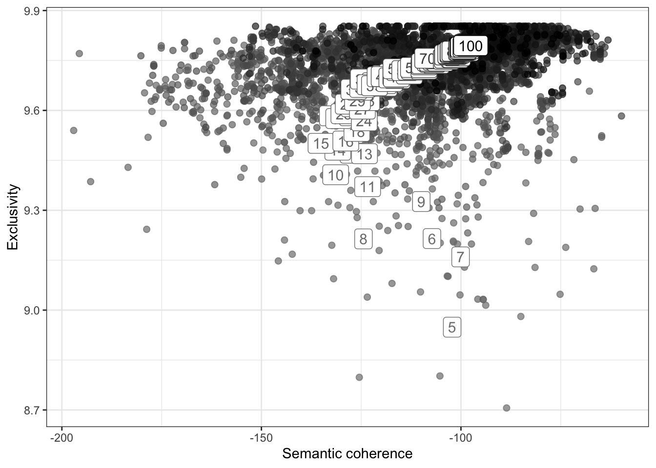
# define range to check for exclusivity and semantic coherence
range <- seq(5, 100, 1)

# calculate exclusivity and semantic coherence
group_means <- k_result %>%
  select(K, exclusivity, semantic_coherence) %>%
  filter(K %in% range) %>%
  unnest(cols = c(exclusivity, semantic_coherence)) %>%
  mutate(K = as.factor(K)) %>%
  group_by(K) %>%
  summarise(
    exclusivity = mean(exclusivity),
    semantic_coherence = mean(semantic_coherence)
  )

# plot semantic coherence and exclusivity
k_result %>%
  select(K, exclusivity, semantic_coherence) %>%
  filter(K %in% range) %>%
  unnest(cols = c(exclusivity, semantic_coherence)) %>%
  mutate(K = as.factor(K)) %>%
  ggplot(aes(semantic_coherence, exclusivity, z = K, color = K)) +
  geom_point(size = 2, alpha = 0.7) +
  geom_label(data = group_means, label = group_means$K, size = 4, show.legend = FALSE) +
  labs(x = "Semantic coherence",
       y = "Exclusivity") +
  theme_bw() +
  theme(legend.position = "none") +
  scale_color_grey(start = .5, end = 0)
# extract k = 7 model
topic_model <- k_result %>%
  filter(K == 7) %>%
  pull(topic_model) %>%
  .[[1]]

topic_model
A topic model with 7 topics, 149 documents and a 306 word dictionary.Inspect Model
# beta (probabilities that each word is generated from each topic)
td_beta <- tidy(topic_model)
td_beta
# A tibble: 2,142 × 3
topic term beta
<int> <chr> <dbl>
1 1 class 1.34e- 67
2 2 class 1.90e- 3
3 3 class 3.68e- 87
4 4 class 4.65e- 3
5 5 class 4.24e- 50
6 6 class 6.12e- 3
7 7 class 1.24e- 17
8 1 classroom 1.16e-101
9 2 classroom 8.67e- 52
10 3 classroom 8.44e-106
# … with 2,132 more rows
# ℹ Use `print(n = ...)` to see more rows# gamma (probabilities that each document is generated from each topic)
td_gamma <- tidy(topic_model, matrix = "gamma",
document_names = rownames(sparse_docs))
td_gamma# A tibble: 1,043 × 3
document topic gamma
<chr> <int> <dbl>
1 1 1 0.00620
2 2 1 0.00914
3 3 1 0.923
4 4 1 0.00906
5 5 1 0.00624
6 6 1 0.0118
7 7 1 0.0283
8 8 1 0.00893
9 9 1 0.00900
10 10 1 0.536
# … with 1,033 more rows
# ℹ Use `print(n = ...)` to see more rows# top terms
top_terms <- td_beta %>%
arrange(beta) %>%
group_by(topic) %>%
top_n(20, beta) %>%
arrange(-beta) %>%
select(topic, term) %>%
summarise(terms = list(term)) %>%
mutate(terms = map(terms, paste, collapse = ", ")) %>%
unnest(cols = c(terms))
top_terms# A tibble: 7 × 2
topic terms
<int> <chr>
1 1 internet, game, adolescent, service, health, demand, user, wellbeing, p…
2 2 relationship, science, satisfaction, student, technostress, competence,…
3 3 internet, satisfaction, relatedness, health, competence, adult, program…
4 4 student, teacher, control, school, education, university, learning, str…
5 5 media, satisfaction, competence, relatedness, influence, motivation, us…
6 6 participant, life, health, user, motivation, faculty, activity, app, ex…
7 7 employee, motivation, relationship, job, workplace, knowledge, relatedn…# top gamma terms
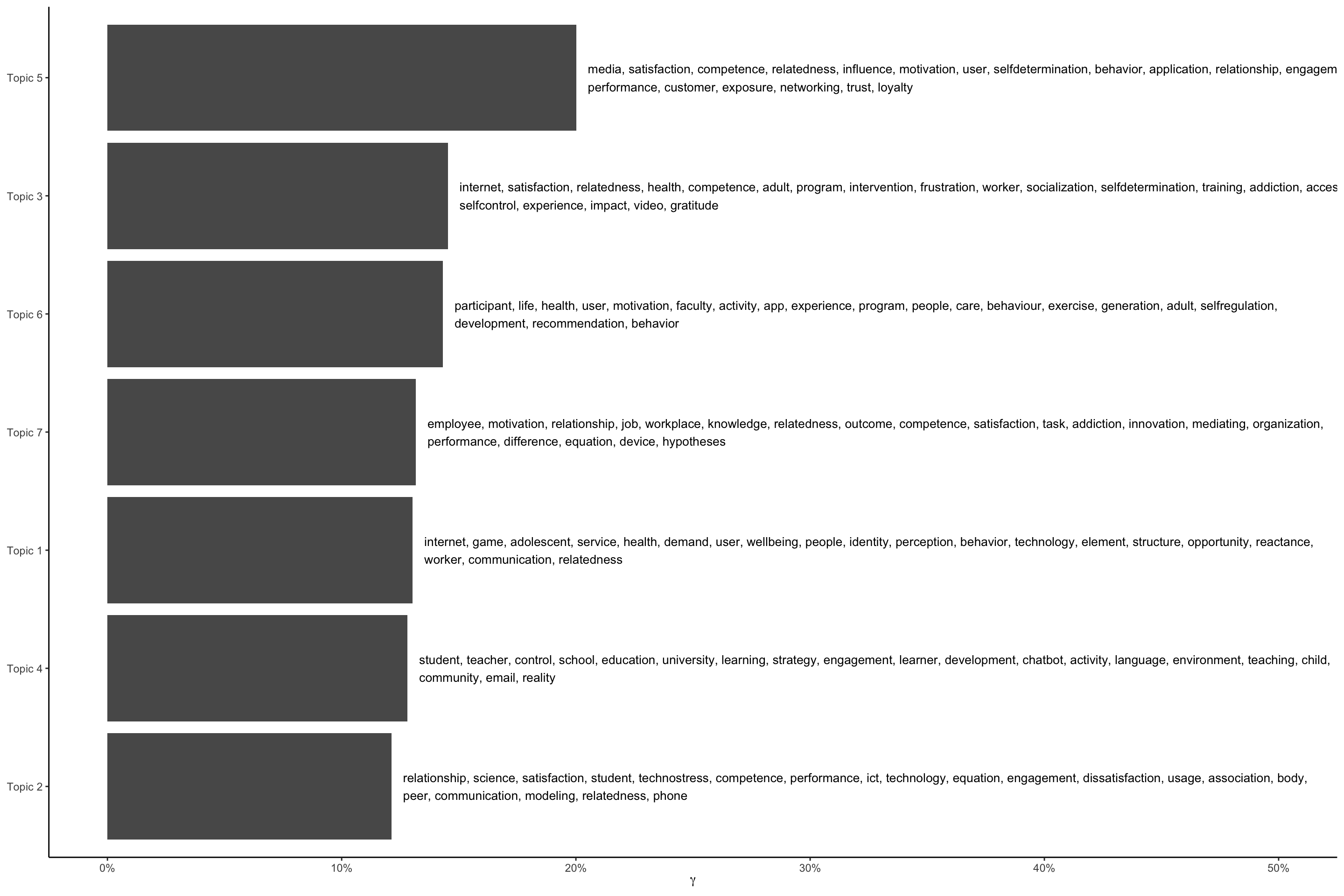
gamma_terms <- td_gamma %>%
group_by(topic) %>%
summarise(gamma = mean(gamma)) %>%
arrange(desc(gamma)) %>%
left_join(top_terms, by = "topic") %>%
mutate(topic = paste0("Topic ", topic),
topic = reorder(topic, gamma))
gamma_terms# A tibble: 7 × 3
topic gamma terms
<fct> <dbl> <chr>
1 Topic 5 0.200 media, satisfaction, competence, relatedness, influence, motiva…
2 Topic 3 0.145 internet, satisfaction, relatedness, health, competence, adult,…
3 Topic 6 0.143 participant, life, health, user, motivation, faculty, activity,…
4 Topic 7 0.132 employee, motivation, relationship, job, workplace, knowledge, …
5 Topic 1 0.130 internet, game, adolescent, service, health, demand, user, well…
6 Topic 4 0.128 student, teacher, control, school, education, university, learn…
7 Topic 2 0.121 relationship, science, satisfaction, student, technostress, com…# plot top gamma terms
gamma_terms %>%
ggplot(aes(topic, gamma, label = str_wrap(terms, width = 170))) +
geom_col(show.legend = FALSE) +
geom_text(hjust = 0, nudge_y = 0.005, size = 3.5) +
coord_flip() +
scale_y_continuous(labels = scales::percent_format(), limits = c(0, .5)) +
labs(x = NULL, y = expression(gamma)) +
theme_classic()
# get top topic (highest probability) per doc
top_classification <- td_gamma %>%
  group_by(document) %>%
  top_n(1, gamma) %>%
  ungroup() %>%
  mutate(doc_id = as.numeric(document))

top_classification
# A tibble: 149 × 4
document topic gamma doc_id
<chr> <int> <dbl> <dbl>
1 3 1 0.923 3
2 10 1 0.536 10
3 14 1 0.952 14
4 15 1 0.884 15
5 18 1 0.728 18
6 19 1 0.948 19
7 21 1 0.953 21
8 40 1 0.572 40
9 43 1 0.329 43
10 71 1 0.927 71
# … with 139 more rows
# ℹ Use `print(n = ...)` to see more rows# add top topic (highest probability) to docs
topic_docs <- inner_join(docs, top_classification) %>%
relocate(topic, gamma, .after = doc_id)
# get top concepts by topic
top_topic_concepts <- topic_docs %>%
select(-concept_id, -concept_score, -concept_lecel, -concept_url) %>%
unnest(all_concepts) %>%
filter(concept_name != "Autonomy") %>%
group_by(doc_id, topic) %>%
arrange(concept_lecel, .by_group = TRUE) %>%
group_by(topic, concept_name) %>%
summarise(n = n()) %>%
arrange(desc(n), .by_group = TRUE) %>%
filter(row_number() %in% 1:3) %>%
mutate(
top_topic_concepts = str_flatten(concept_name, collapse = ", "),
topic = str_c("Topic ", topic) %>% as_factor()) %>%
nest(all_concepts = c(concept_name, n))
top_topic_concepts <- left_join(gamma_terms, top_topic_concepts)
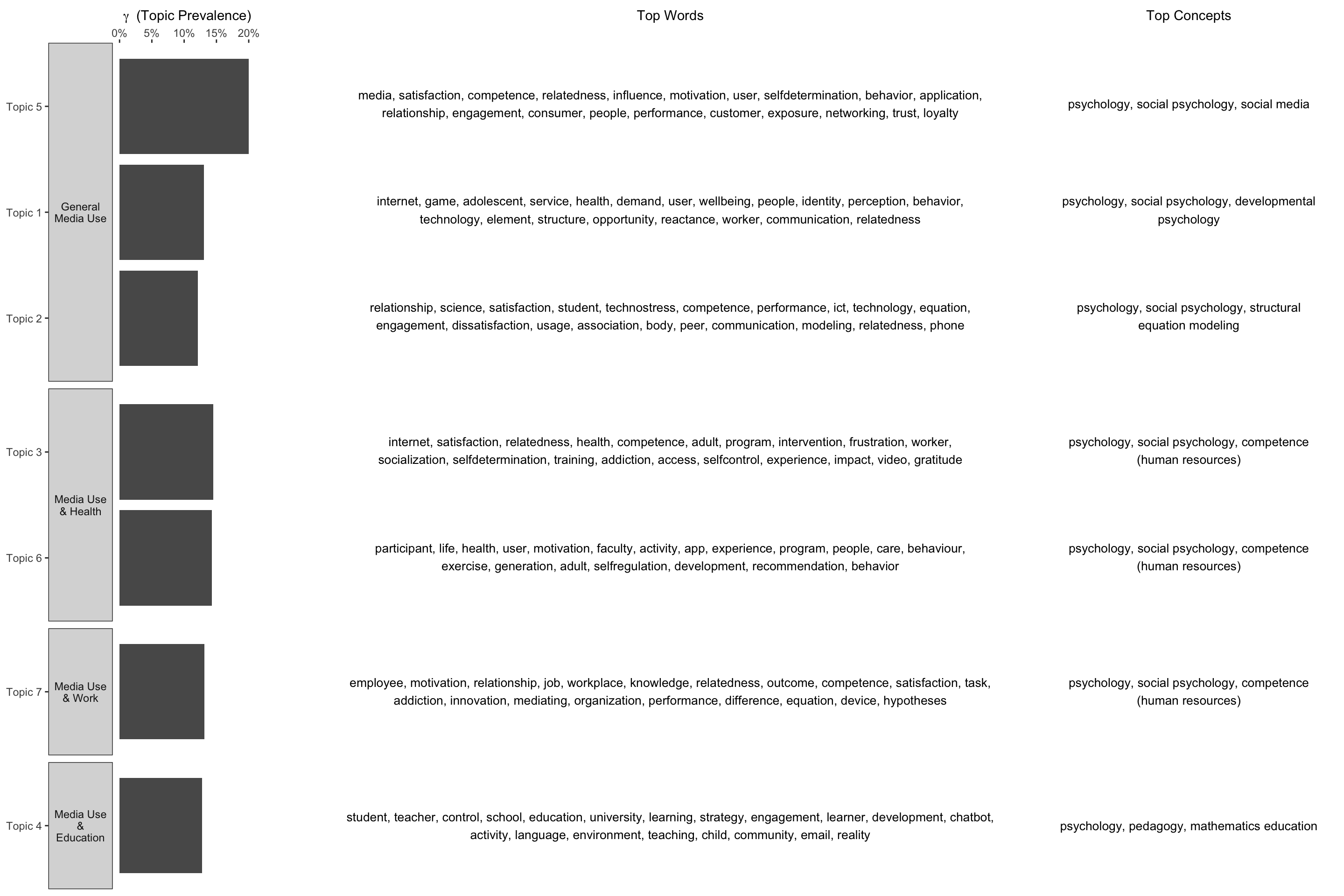
# add manual topic labels after inspecting concepts and top words
topic_labels <-
tribble(
~ topic, ~ label,
"Topic 1", "General Media Use",
"Topic 2", "General Media Use",
"Topic 3", "Media Use & Health",
"Topic 4", "Media Use & Education",
"Topic 5", "General Media Use",
"Topic 6", "Media Use & Health",
"Topic 7", "Media Use & Work",
) %>%
mutate(
topic = as.factor(topic),
label = as.factor(label)
)
# order by sum of gamma by manual topic
top_topic_concepts_plot <- left_join(top_topic_concepts, topic_labels) %>%
group_by(label) %>%
mutate(
order = sum(gamma)
) %>%
ungroup() %>%
mutate(label = fct_reorder(label, order, .desc = TRUE))
# plot
p1 <- top_topic_concepts_plot %>%
ggplot(aes(topic, gamma)) +
geom_col(show.legend = FALSE) +
coord_flip() +
scale_y_continuous(labels = scales::percent_format(),
limits = c(0, .21), position = "right",
breaks = c(0, .05, .1, .15, .2)) +
labs(x = NULL, y = expression(gamma ~ " (Topic Prevalence)")) +
facet_grid(rows = vars(label), scales = "free_y", space = "free_y",
labeller = labeller(label = label_wrap_gen(10)),
switch = "y") +
theme_bw() +
theme(strip.text.y.left = element_text(angle = 0),
panel.grid = element_blank(),
panel.border = element_blank())
p2 <- top_topic_concepts_plot %>%
ggplot(aes(topic, gamma)) +
geom_text(aes(label = str_wrap(terms, width = 120), y = 0), hjust = 0.5, size = 3.5) +
coord_flip() +
scale_y_continuous(position = "right") +
facet_grid(rows = vars(label), scales = "free_y", space = "free_y") +
theme_bw() +
ylab("Top Words") +
theme(axis.line = element_blank(),
axis.text.x = element_text(colour = "#ffffff"),
axis.text.y = element_text(colour = "#ffffff"),
axis.ticks = element_blank(),
axis.title.y = element_blank(),
strip.background.y = element_blank(),
strip.text.y = element_blank(),
panel.grid = element_blank(),
panel.border = element_blank())
p3 <- top_topic_concepts_plot %>%
ggplot(aes(topic, gamma)) +
geom_text(aes(label = str_wrap(str_to_lower(top_topic_concepts), width = 45), y = 0),
hjust = 0.5, size = 3.5) +
coord_flip() +
scale_y_continuous(position = "right") +
facet_grid(rows = vars(label), scales = "free_y", space = "free_y") +
theme_bw() +
ylab("Top Concepts") +
theme(axis.line = element_blank(),
axis.text.x = element_text(colour = "#ffffff"),
axis.text.y = element_blank(),
axis.ticks = element_blank(),
axis.title.y = element_blank(),
strip.background.y = element_blank(),
strip.text.y = element_blank(),
panel.grid = element_blank(),
panel.border = element_blank())
ggarrange(p1, p2, p3,
ncol = 3, nrow = 1,
widths = c(.6 , 1.7, .7))